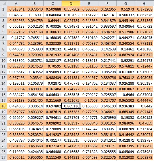
Sometimes when you look at large amounts of data on the screen in Excel it can be difficult to read and comprehend because of the uniform color (white). Through the use of conditional formatting and formula you can add alternate row/column shading.
1. In an Excel spreadsheet, select the data.
2. On the “Home” tab, click “Conditional Formatting” and choose “New Rule.”
3. In the “New Formatting Rule” dialog box, select “Use a formula to determine which cells to format.”
4. In the “Format values where this formula is true:” field, type = mod(row(),2)=1. This formula means that whenever the row number is odd, change the format. There could be similar versions which you can use:
– To change the coloring of even rows change the formula to = mod(row(),2)=0
– To change the coloring of even columns change the formula to = mod(column(),2)=0
– To change the coloring of every third row change the formula to = mod(row(),3)=0
5. Click “Format,” and then format the cells as you choose. The “Fill” tab will allow for the choice of row/column color.
6. Click “OK” twice to close the dialog boxes.
These instructions, along with illustrations, can also be found in SharePoint > Software Users Group > Shared Documents > Excel > Shading Alternate Rows-Columns.
This tip was originally taken from http://www.exceloogle.com/2013/06/trick-how-to-shade-alternate-rowscolumns.html?goback=.gde_4148190_member_253245093.